Algorithms and Data Structures Series: Big O Notation
May 3, 2022 - Geison BiazusThis is the first post in a series of posts about algorithms and data structures that I'm going to write. But before digging into this topic it is important to know about the Big O notation as it is the basis for measuring the complexity of algorithms allowing us to decide which is the best algorithm or data structure for every specific case.
Contents
- What is the Big O Notation
- Identifying the time complexity
- Identifying the space complexity
- Final thoughts
- Sources
What is the Big O Notation
Big O is part of a family of mathematical notations invented by Paul Bachmann and Edmund Landau. Wikipedia states that "...big O notation is used to classify algorithms according to how their run time or space requirements grow as the input size grows...". In other words, it is a way to classify the complexity and scalability of the code based on how the number of operations increases when the input size grows.
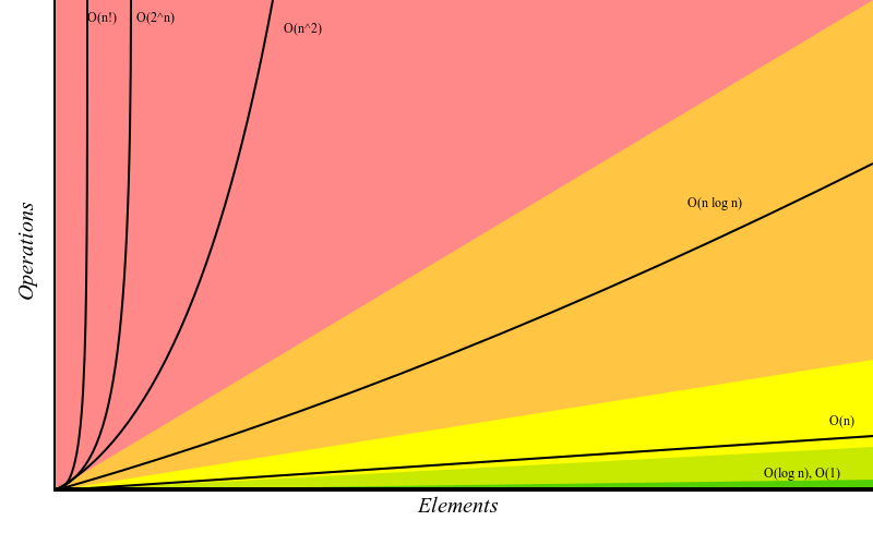
Big O is expressed in a simple and common notation that makes it easier for developers to discuss the algorithm complexities and find the optimal solutions for both the implementation and the choice of the best fitting data structure for a specific problem. The following figure visually shows how each of the most common complexities compares to each other:
Two kinds of complexity can be classified with Big O:
- Time complexity - Classifies how long the algorithm takes to run based on the input size
- Space complexity - Classifies how much extra memory the algorithm uses based on the input size
The code examples used in the next sections of this post are written using the Go programming language, but its syntax is simple enough that can be easily understood, and they can be implemented using any language.
Identifying the time complexity
To identify the time complexity of an algorithm, we go line by line calculating its complexity. The following example shows this process. You can see the complexity of each line as a comment at the end of the same line.
 1func example(num, times int) int {
 2  result := num         // O(1)
 3  result = result + num // O(1)
 4
 5  for i := 0; i < times; i++ { // O(n)
 6    result *= num // O(1)
 7    result *= 2   // O(1)
 8  }
 9
10  return result // O(1)
11}
Looking at this example, you can notice that we marked the lines 2, 3, 6, 7, and 10 as having a time complexity of O(1). This means that on these lines, it doesn't matter the input that is given, it will always take the same time to compute, so we say that the complexity of these lines is constant.
Line 5, on the other hand, is marked as O(n). The n here means the size of the input, in this case, the times argument. The complexity O(n) means that the amount of operations that run on this line is proportional to the size of the input, so we say that the complexity of this line is linear.
Now if we calculate the complexity of the whole function we end up with this:
O(1 + 1 + n * (1 + 1) + 1)
or
O(3 + 2n)
To calculate the final Big O for any function, we always drop the constants as they are not relevant on a high scale. So instead of classifying the function as O(3 + 2n) we simply classify this function as O(n) because what matters here is that the time complexity of the function grows proportional to the size of the input.
Examples of common time complexities
Now we'll see some examples of the most common time complexities and how they are classified. We will start with the O(1), O(n), and O(n^2) complexities as they are easier to identify.
O(1) - Constant
We say that an algorithm is "constant", or O(1), when its complexity doesn't change, no matter the input that is given:
1func add(a, b int) int {
2  return a + b
3}
The number of lines is not taken into consideration here. As long as the input does not affect the number of operations, the algorithm's complexity is O(1).
O(n) - Linear
An O(n) algorithm, also referred to as "linear", happens when the number of operations is proportional to its input size:
1func sum(values []int) int {
2  result := 0
3
4  for _, v := range values {
5    result += v
6  }
7
8  return result
9}
It doesn't matter if the input is a list, a string, or a number. As long as the number of operations grows accordingly to the input size, it is considered O(n). Usually, when we have a loop, our algorithm has linear complexity.
Sometimes the loop exits prematurely, even so, we always consider the worst-case scenario:
1func includes(values []int, val int) bool {
2  for _, v := range values {
3    if v == val {
4      return true
5    }
6  }
7  return false
8}
The above example is also considered O(n) as it is impossible to know where in the list the value is, or even if it is included.
A recursive algorithm also can lead to a linear complexity:
 1func includes(values []int, val, index int) bool {
 2  if index >= len(values) {
 3    return false
 4  }
 5
 6  if values[index] == val {
 7    return true
 8  }
 9
10  return includes(values, val, index+1)
11}
The example above has also an O(n) complexity as it makes use of recursion to loop through the input searching for the value.
An algorithm that has more than one loop is also considered linear as long as the loops are not nested:
 1func sumAndMultiply(values []int) (int, int) {
 2  sum := 0
 3  for _, v := range values {
 4    sum += v
 5  }
 6
 7  product : = 0
 8  for _, v := range values {
 9    product *= v
10  }
11
12  return sum, product
13}
This example loops through the input twice so its complexity would be something like O(2n). But as mentioned before, we always cut the constants so we still consider this algorithm as having a complexity of O(n).
Iterating through half of a list is also considered O(n):
1func isPalindrome(str string) {
2  for i := 0; i < len(str) / 2; i++ {
3    j := len(str) - 1 - i
4    if str[i] != str[j] {
5        return false
6    }
7  }
8  return true
9}
This example is similar to the one with two loops. Although the calculated complexity would be something like O(n/2), as we cut the constants we consider it as O(n). On a large scale, the constants are not relevant, therefore this algorithm is considered linear as its number of operations still grows proportionally to the input size.
O(n + m)
When the algorithm complexity is influenced by more than one input, we use more than one variable to classify it:
 1func merge(a, b []int) []int {
 2  result := []int{}
 3
 4  for _, value := range a {
 5    resut = append(result, value)
 6  }
 7
 8  for _, value := range b {
 9    resut = append(result, value)
10  }
11
12  return result
13}
In the previous example, the two lists are traversed entirely, and as their sizes are independent of each other, we classify this function as having a complexity of O(n + m).
O(n^2) - Quadratic
An algorithm is O(n^2) or "quadratic" when for every item of the input, the whole input is traversed. It happens when we have nested loops:
 1func hasDuplicates(list []int) bool {
 2  for i := 0; i < len(list)-1; i++ {
 3    for j := i + 1; j < len(list); j++ {
 4      if i != j && list[i] == list[j] {
 5        return true
 6      }
 7    }
 8  }
 9  return false
10}
In this example, for every new element in the input list, a new loop is performed, therefore the time complexity of this algorithm is O(n^2). This is a very common complexity found in naive code and unless the input is known to be small, it should be avoided and optimized as it can become very slow.
O(n * m)
When we have nested loops but with different inputs, we use different variables to classify each one of the inputs:
 1func intersection(a, b []int) []int {
 2  result := []int{}
 3
 4  for _, v1 := range a {
 5    for _, v2 := range b {
 6      if v1 == v2 {
 7        resut = append(result, value)
 8      }
 9    }
10  }
11
12  return result
13}
Here, for every element of a we traverse b, consequently we can classify this algorithm as having an O(n * m) complexity.
From this point on, the complexities are still commonly found in algorithms, but they are a little harder to identify.
O(log n) - Logarithmic
This complexity is commonly found in binary trees or binary searches. It happens, for example, when we don't need to traverse the whole list to find the desired value, instead, we can divide the list in two until we find what we're looking for. In these cases we say that the algorithm has an O(log n) complexity or it is "logarithmic":
 1func binarySearch(list []int, value int) bool {
 2  if len(list) == 1 {
 3    return list[0] == value
 4  }
 5
 6  if len(list) == 0 {
 7    return false
 8  }
 9
10  mid := len(list) / 2
11
12  if value < list[mid] {
13    return binarySearch(list[:mid], value)
14  } else {
15    return binarySearch(list[mid:], value)
16  }
17}
In this example, we have an implementation of a binary search. A sorted list is given as the input. To check if the desired value is included in the list, the list is split into two halves. If the value is smaller than the middle element, the first half is considered, otherwise the second half. It does that recursively until the value is found or the end is reached. For example, if we want to check if 3 is included in the list [1, 2, 3, 6, 7, 9, 10, 15], the list will be split the list as follows:
       1 2 3 6 7 9 10 15
      /                 \
   1 2 3 6           7 9 10 15
  /      \
1 2      3 6
        /   \
      (3)    6
To find a value in a list of 8 elements, three splits happen. The number of operations can be found based on the input length with a logarithm function. If we calculate Log 8 the result is 3. That's why we classify this complexity as O(log n).
The result of the log function is not always exact. For example Log 7 is 2.80. A list with 7 elements still does 3 operations, but we still classify the algorithm as O(log n) because the number of operations grows accordingly to the input in a logarithmic proportion.
O(n log n) - Log-linear
The O(n log n) complexity happens when we have log n interactions, but for every interaction, we traverse the whole list with an additional n complexity. This is the complexity of the sorting algorithms Merge Sort, Quick Sort, and Heap Sort. I'll bring some examples of algorithms with this complexity in a future post when I write about sorting algorithms.
O(2^n), O(n!), and beyond
There are complexities worse than O(n^2) like O(2^n) and O(n!). We won't get into details on those here. If you're interested in knowing more about these complexities, as well as seeing some examples, you can check the article 8 time complexities that every programmer should know by Adrian Mejia.
In summary, except in cases where the input is known to be small we should try not to exceed the O(n) complexity, with some exceptions of O(n log n). Many times we can decrease time complexity by increasing space complexity using techniques like Divide and Conquer and Dynamic Programming, and if we have the memory to spare, they are worth the trade-off.
Identifying the space complexity
The space complexity can also be classified using the Big O notation. It measures the amount of extra memory an algorithm needs to complete its execution. We can identify the space complexity by looking at new variables, data structures and function calls inside of the algorithm.
Examples of common space complexities
O(1) - Constant
When the additional space used by the algorithm is constant no matter the input size, it is classified as O(1) or "constant" complexity:
1func sum(values []int) int {
2  result := 0
3
4  for _, v := range values {
5    result += v
6  }
7
8  return result
9}
This example has an O(n) time complexity, but it creates only one new variable which is not affected by the input size, therefore its space complexity is O(1).
O(n) - Linear
When the new amount of memory used by the algorithm grows in the same proportion as the input, we classify it as having a space complexity of O(n) or "linear".
1func addItem(list []int, item int) []int {
2  result := []int{}
3
4  for _, v := range values {
5    result = append(result, v)
6  }
7
8  return append(result, list)
9}
In this immutable function to add an item to a list, a new list is generated of the same size as the input. That makes its space complexity be O(n).
Function calls also increase the amount of memory necessary for an algorithm. That's why recursive functions usually receive an O(n) space complexity:
 1func includes(values []int, val, index int) bool {
 2  if index >= len(values) {
 3    return false
 4  }
 5
 6  if values[index] == val {
 7    return true
 8  }
 9
10  return includes(values, val, index+1)
11}
The recursive "includes" example does not create any new variable, but as the number of times it calls itself recursively is the same as the length of the input, it has a linear space complexity, or O(n).
O(n^2) and beyond
As we can see, the same rules we use to detect the time complexity, we do for the space complexity. For an O(n^2) algorithm, the amount of memory grows n * n times. An O(log n) function grows its memory in a logarithmic proportion, and so on.
Final thoughts
Every programmer has an idea of how to recognize when an algorithm is optimized, but having a way to classify these complexities promotes the sharing of this information and makes conversations and discussions easier.
Knowing the Big O notation is very important when choosing a data structure or an algorithm. Some operations have different complexities in different data structures and we should be able to decide the best fit for our problems.
My intention with this post is to give you a basic understanding of the different algorithm complexities as they will be used in the posts to come. I hope you enjoyed it and learned something new.